Abstract
Dynamic Light Scattering is commonly used to rapidly measure the hydrodynamic size and size dispersity of nanoparticles in suspension. Several commercial DLS instruments exist, using a range of illumination wavelengths and detection angles. These varying instrument specifications have an effect on the measured nanoparticle size and polydispersity index, even for relatively monodisperse nanosuspensions. Here, we explain how results from DLS instruments at different wavelengths and scattering angles are related using practical examples, computer simulations and established light scattering theory, in the context of recently introduced novel Spatially Resolved DLS technology using Near InfraRed light.
Introduction
Dynamic Light Scattering (DLS) is a technique that measures the hydrodynamic diameter of nano-particles in suspensions by analyzing their Brownian motion based on measurement of intensity fluctuations of scattered light. In various industry and academic R&D/QC labs, DLS is used to rapidly measure the size and size dispersity of nanoparticles (NPs). The use of DLS in NP sizing is highly convenient, as it is simple to set up, is based on first principles (requiring no calibration), needs relatively little sample preparation and allows relatively fast measurement (the latter two depending on the instrument used) [1]. However, DLS has its limitations as an NP characterization technique. For instance, its resolution in distinguishing individual particle populations is low, compared to more laborious, complex particle counting techniques. DLS is thus best suited for fast screening, rather than highly resolved studies on details of the particle size distribution (PSD).
At InProcess-LSP, efforts focus on helping customers upgrade their R&D labs and manufacturing plants from standard off-line DLS systems to continuous, inline, real-time process monitoring systems based on Spatially Resolved DLS (SR-DLS, implemented in the ‘NanoFlowSizer’). Although SR-DLS still employs conventional DLS theory, the advanced depth-resolved character of the measurement allows for real-time NP size and dispersity measurements in flowing and turbid suspensions [2]. This improvement allows using SR-DLS as a Process Analytical Technology (PAT) tool for inline NP sizing.
Since DLS is widely recognized as NP sizing technique of choice, various DLS instruments are commercially available, each with its own technical specifications. Important parameters such as the wavelength of the light (λ) and the angle at which scattered light are detected (θ) vary significantly between instruments. An often-overlooked, yet vital question here is: How can particle size characteristics measured using different DLS instruments be compared to each other?
The NanoFlowSizer (NFS) system, specifically designed for flexible measurements for a broad range of (flow) geometries and sample cells, operates at full backscattering 180⁰. Furthermore, it employs Near InfraRed light (~1300 nm center wavelength). In this article, we aim to clarify how particle size data from different conventional DLS systems can be compared to each other and to the data collected using the novel (NIR) SR-DLS technology.
(Spatially Resolved) Dynamic Light Scattering and the NanoFlowSizer
Standard DLS measures fluctuations in the intensity of scattered laser light due to Brownian diffusion of NPs (see Fig.1A, left panel). The spectrum of these intensity fluctuations reflects the (distribution of) the NPs diffusion coefficient D, and is typically analyzed using the intensity ‘Auto Correlation Function’ (ACF) [1]. For particles of a single hydrodynamic size d, the ACF decays exponentially at a rate proportional to the diffusion coefficient D. Since the latter is related to the size via the Stokes-Einstein relation [3], D∝T/(η d) with T the temperature and η the solvent viscosity, the particle size can be obtained when temperature and viscosity are known. As detailed later, for suspensions with NPs having a distribution of sizes, the ACF can be analyzed to obtain intensity-weighted size characteristics either as the mean ‘Z-av’ size and a polydispersity index representing the width of the distribution, or as intensity-based PSD from more advanced ACF analysis.
For conventional DLS, inline measurements at industrially relevant flowrates are not possible: standard DLS requires (nearly) static conditions to ensure that the measured intensity fluctuations are solely due to NP diffusion, while it is also limited to low turbidity samples to avoid multiple scattering. This is often not the case in industry, limiting efficient use of standard DLS in these situations.
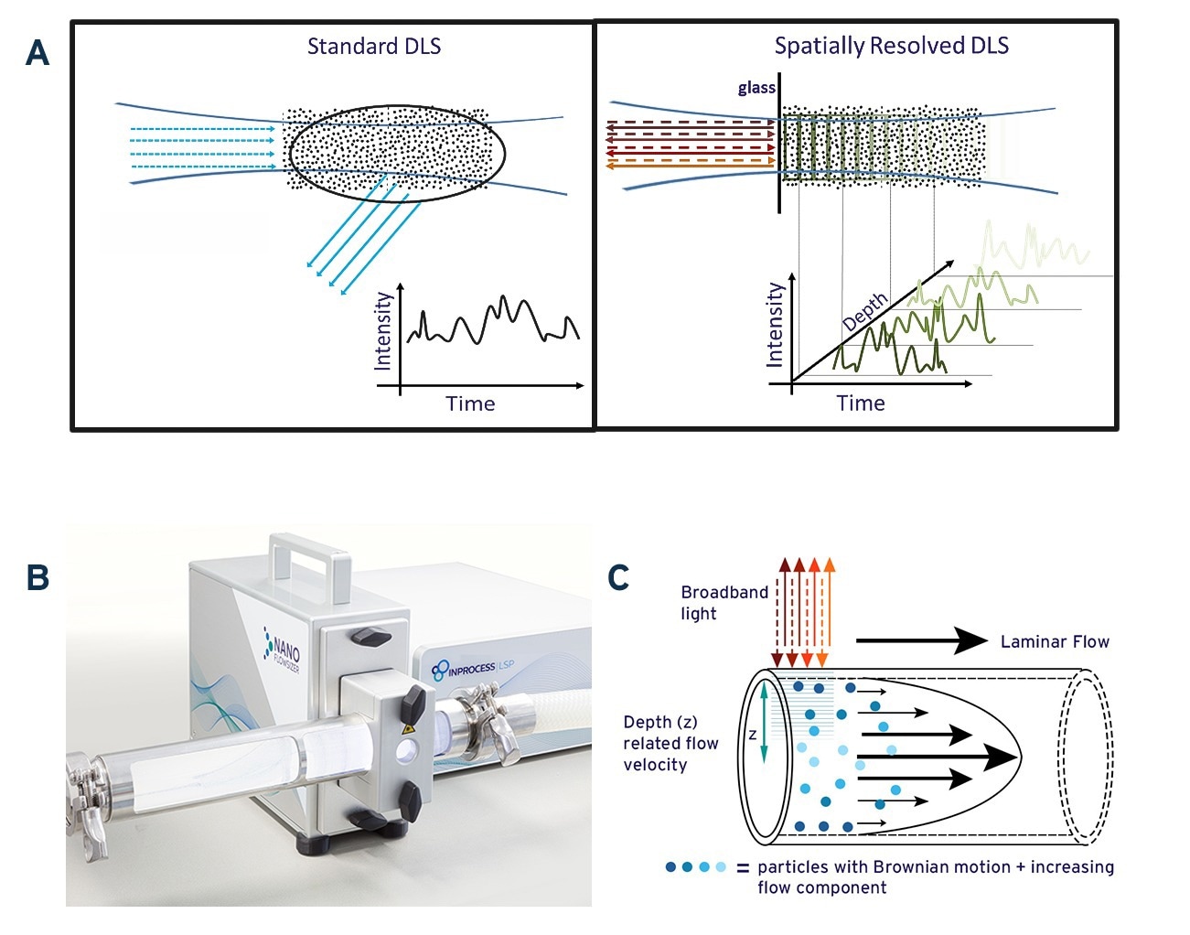
Fig. 1A: Schematic illustration of standard DLS measurement and Spatially Resolved-DLS. 1B: The NanoFlowSizer, a PAT device based on SR-DLS to measure turbid nanosuspensions in flow. 1C: Representation of particle motion during laminar pipe flow of a nanosuspension. Broadband illumination from the NFS probe and backscattering are also indicated. Source: InProcess-LSP
To overcome these limitations, InProcess-LSP developed the NanoFlowSizer (NFS) (Fig.1B) [2]. It uses ‘Low Coherence Interferometry’ with broadband Near InfraRed (NIR) light (~1300nm center wavelength), which enables Spatially Resolved Dynamic Light Scattering (SR-DLS). This method instantaneously resolves scattered light and its fluctuations from different depths in the sample (Figure 1A, right panel) providing information on particle motion both due to flow and diffusion. Both contributions can be extracted from SR-DLS measurements and used to obtain size characteristics in laminar flows up to at least 300 L/h (Figure 1C). Additionally, automatic ‘spatial filtering’ excluding multiple scattered light enables measuring samples with turbidity levels far exceeding the limit for traditional DLS. The NFS can be applied from small-scale laboratory/pilot scale processes to full-scale production pipelines by simply switching the measurement module used.
Besides the spatial resolution, the use of NIR wavelengths further enhances the turbidity range since turbidity decreases as 1/λ4, in other words, the mean path length over which photons scatter increases as λ4. Besides this advantage, the use of NIR also reduces absorption that can be encountered in DLS and also avoids possible influence of fluorescence, which may interfere with DLS measurements using visible light. In the following it is explained that besides these advantages, use of NIR light also has other advantages, regarding the interpretation of intensity-based DLS results.
Scattering Intensity in DLS – influence of particle size and detection angle θ
Light that is scattered by spherical particles can be described using various well-established theories [4]. The most important parameter in these theories is the ratio d/λ' of the particle diameter d and the wavelength of light in the medium, λ'=λ/ns (λ is the wavelength in vacuum, ns the solvent refractive index (RI)). The most complete model, for scattering at any relative size d/λ', is Mie theory [5]. It covers the regime from particles much smaller than the wavelength (d/λ' < 0.1), known as Rayleigh Scattering, to sizes comparable or larger than the wavelength (‘Mie’ regime).
The Rayleigh and Mie regimes show characteristic differences in overall scattering intensity and how the scattered intensity depends on the scattering angle. In Fig.2A, the differences in angular dependence are shown using a polar intensity plot for different size/wavelength ratios d/λ'. In the Rayleigh regime (d/λ' < ~ 0.1) scattering is isotropic, independent of angle. For larger size ratio, d/λ' = 1, scattering becomes more biased in the forward direction (anisotropic), a characteristic feature of the ‘Mie’ regime due to diffraction effects. For larger sizes, the anisotropy increases and the angular pattern develops several maxima and minima, as visible for the size ratio d/λ' = 10. The anisotropy is important for (PAT) nanoparticle sizing methods: backscattered intensity measurements (at θ~180⁰) suffer much less from the dominant scattering from large particles compared to measurements for θ<90⁰. This in principle allows better-resolved measurement of more polydisperse suspensions containing both large and small particles.
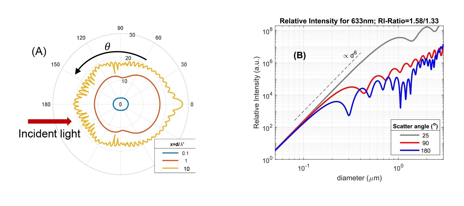
Fig. 2A: Angular intensity pattern of light scattered from a single particle, based on Mie theory. Data are shown for three ratios of particle size d and incident wavelength in the medium (x = d/λ'). Ratio of particle/solvent refractive index is 1.58/1.33. The radial axis is scaled logarithmically and the red arrow indicates the direction of the incident light. 2B: Scattered intensity versus particle size for three scattering angles (wavelength λ=633 nm, RI-ratio 1.58/1.33). Source: InProcess-LSP
The change in intensity and anisotropy on changing the size/wavelength ratio are more directly visible when the intensity is plotted versus size for a specific instrument wavelength at different angles, as in Fig.2B for incident light of 633 nm (commonly used in standard DLS instruments). Firstly, in the Rayleigh regime d/λ' < ~ 0.1 (practically for sizes <~ 100nm in Fig. 2B) the data show the well-known strong increase of intensity with size, as ∝d6 or volume2, regardless of the angle. Entering the Mie regime, for sizes approaching ~λ/2, scattering in the backward direction (~θ>90⁰) levels of and shows maxima and minima versus size, while in the forward direction (θ<30⁰) the ∝d6 intensity increase continues up to sizes exceeding the wavelength. For ~633nm instruments, measuring low-medium refractive index particles, the first minimum for θ=180⁰ occurs already around a particle size of 300nm. It is exactly this variation of scattering intensity versus size that makes cross-interpretation of intensity-based DLS results difficult.
Scattering Intensity in DLS – Influence of wavelength λ and suspension refractive indices.
Since the scatter intensity depends on the size/wavelength ratio, differences also appear when comparing the scattering in a certain direction as a function of particle size for instruments using different wavelengths. This is shown in Fig.3A for backscattering at three wavelengths. The onset of Mie scattering is visible for particle diameters around 0.2λ and obvious for sizes around 0.5λ. Use of a larger wavelength thus ‘delays’ the onset of Mie scattering to larger particle sizes, which offers the benefit of particle size measurements for larger particles without effects of Mie ‘resonances’. For the SR-DLS-based NanoFlowSizer using 1300 nm as center wavelength, the larger wavelength thus not only helps in measuring turbid suspensions, but also in a more direct interpretation of intensity based Z-av and PdI results in terms of Rayleigh Scattering for a larger size regime.
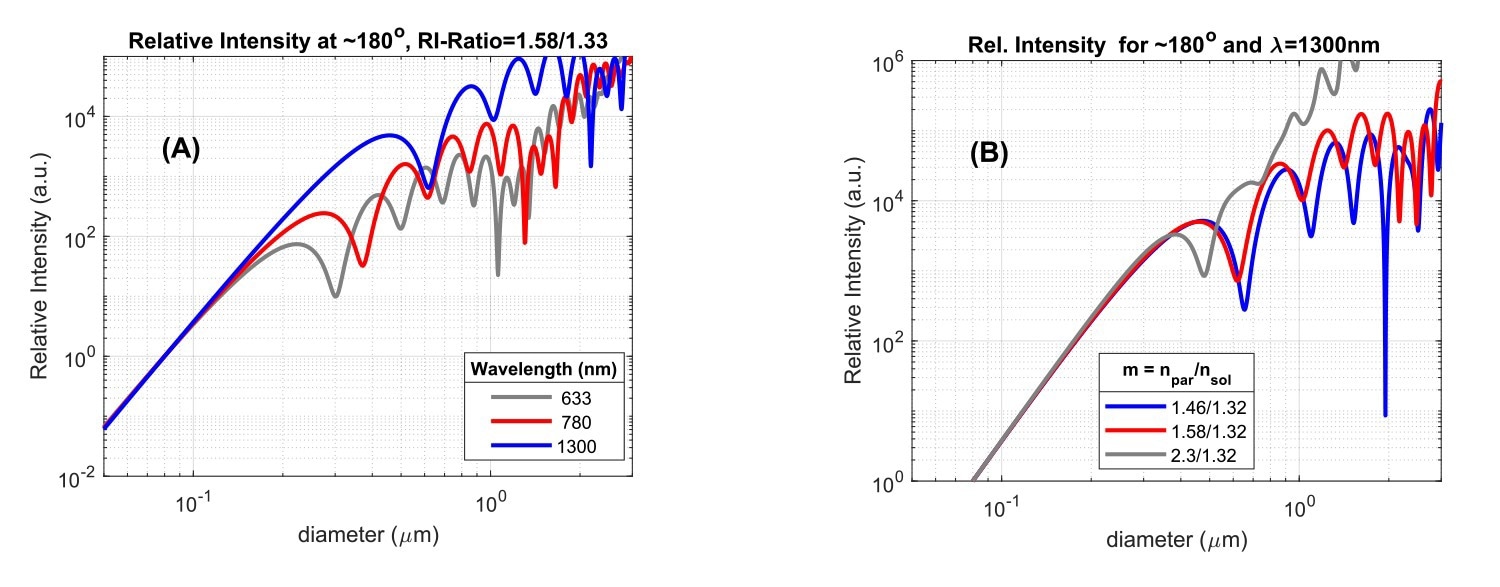
Fig. 3A: Scattered intensity versus particle size, for three wavelengths of incident light, for a particle/solvent RI-ratio of 1.58/1.33, and scattering detected at an angle of ~180⁰. Fig. 3B: Backscattered intensity (θ=180⁰) at λ=1300 nm versus particle size for three particle/solvent RI-ratios. Intensity units are arbitrary and curves are scaled to the same value at d=0.1mm. The absolute scattering level at this value decreases from grey to blue in (A) and (B). Source: InProcess-LSP
Besides angle and wavelength, the last important parameter that affects the scattering is the ratio between particle Refractive Index (RI) and solvent RI (the RI-ratio, m=np/ns). Notably, at fixed solvent RI, the onset of Mie resonances for particles with larger RI occurs for smaller sizes compared to that for lower RI particles. This is shown in Fig.3B for backscattered light at 1300nm (representing the NFS), both for lipid droplets in water (m = 1.46/1.32), polystyrene particles (m = 1.58/1.32), and a large RI-ratio approximating titania NPs in water (m=2.30/1.32). Beyond the Rayleigh regime (here d > ~300 nm) the intensity is significantly impacted by the RI-ratio. Note that the typical RI for hydrophobic ‘Active Pharmaceutical Ingredient’ NPs (present in various nanomedicines), is often very similar to that of polystyrene (Cao et al., 2009). The dependence of Mie scattering on the RI-ratio shown in Fig.3 is the reason why conversion of traditional intensity-based DLS size characteristics to volume-based data generally requires the user to input accurate particle RI, besides the usual solvent RI information. However, when the size range of intensity PSD’s lies in the Rayleigh regime, knowledge of the particle RI is in fact not required for volume conversion, as in that case direct conversion based on I∝d6 can be employed.
Intensity-based size distributions – Practical examples
Due to the variations in scattering intensity shown above, in intensity-based size measurements (as done by default in DLS), each size bin of a Particle Size Distribution (PSD) contributes an intensity that depends on the instrument's detection angle and wavelength. For a specific volume PSD, with a volume mean size dv, one can calculate directly the theoretical Intensity PSD and compare it to the intensity PSD obtained from DLS analysis for different instruments (using simulated DLS correlation functions, see ‘Methods’). Fig 4A shows model volume-based PSD’s along with their corresponding theoretical and ‘DLS’ intensity PSDs in Figs 4B,C, for polystyrene particles in water (m ~1.58/1.33) at (nearly) full backscattering. The PSDs in Fig.4A has a Coefficient of Variation (CoV) of 0.32. For small values, the CoV is linked to the DLS Polydispersity Index (PdI) as (CoV)2≃PdI, the used value would thus translate to a PdI of 0.1. This is typically taken as the limit for considering NPs as monodisperse.
The theoretical intensity PSDs in Figs 4B,C show that for NPs with a smooth volume PSD and CoV = 0.32, significant Mie resonances occur in the PSD for a mean size dv somewhat less than half the wavelength. For an instrument using λ=633nm (and θ=173o, Fig 4C), this occurs already for dv > ~200nm, while for the NFS, operating at 1300nm, this is delayed to sizes >~400nm. Turning to the corresponding ‘DLS’ intensity distributions (solid lines in Fig.4BC), it is clear that PSD analysis schemes based on the DLS autocorrelation function give a smoothed representation of the true intensity distribution and do not capture the intensity minima and maxima in the Mie regime. Therefore DLS intensity-based data covering the Mie regime should not be converted naively to volume PSD using a ‘Mie scaling factor’, as this will yield artificial peaks in volume PSDs. In the NFS XsperGo software, a dedicated method is implemented to avoid such volume conversion artefacts.
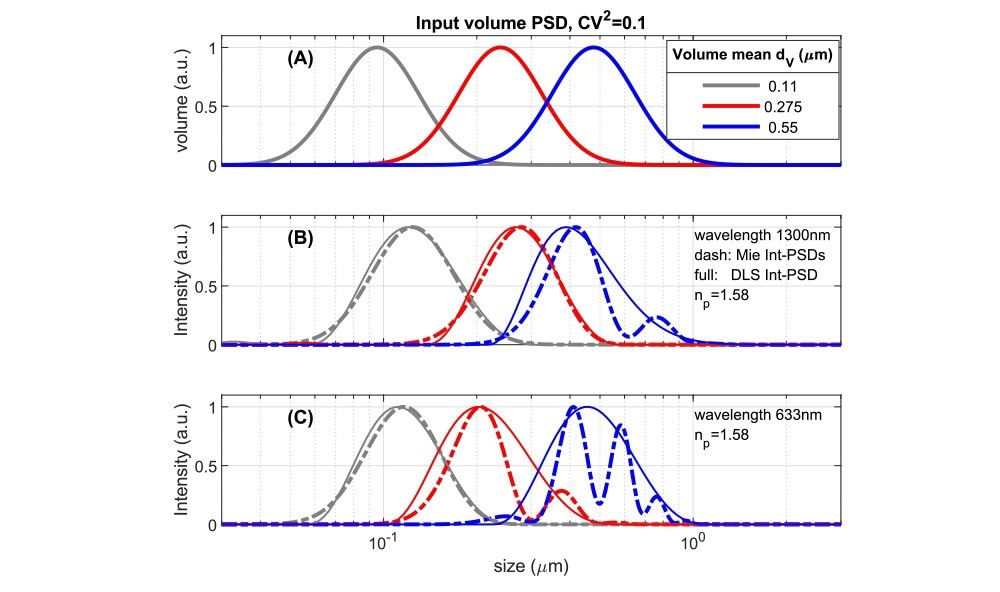
Fig. 4 Comparing volume PSDs with instrument dependent Intensity PSD’s for suspensions with an RI-ratio ~1.58/1.33 representing polystyrene or some pharmaceutical NPs in water. A: Lognormal volume PSD’s used as input to calculate results in 4B,C. 4B: Intensity-based size distributions for 1300nm, 180⁰ backscattered light. Dashed lines are calculated directly from the inputs of 4A using Mie theory. Full lines are ‘measured’ DLS size PSD’s obtained from simulated DLS correlation functions (see ‘Methods’). 4C: as Fig 4B but for a wavelength of 633nm, backscattered at 173⁰. Source: InProcess-LSP
Comparing Intensity-based DLS mean and polydispersity data
The most commonly used size characteristics in DLS are the intensity-based ‘harmonic mean’ Z-av and the associated Polydispersity index PdI, obtained from fitting the logarithm of the correlation function to a second-order polynomial [7], see also [8]. Different intensity weights in DLS correlation functions for different instruments (underlying the differences in Fig 4B,C) also cause different Z-av and PdI data.
Figs. 5A-D highlights these differences for NPs with low RI-ratio (e.g. lipid droplets/NPs, Fig5A, B) and for higher RI-ratio (Fig 5C,D). For both RI-ratios a comparison is made between 1300nm and 630nm (near) backscattering systems, both for Z-av data, grouped into different CoV values in Fig5.A,C, and for the PdI data, grouped into different mean sizes dv in Fig.5B,D. The Z-av comparison in Fig5A,C shows that for ~110nm particles, the difference between Z-av size and dv increases with polydispersity (CoV), somewhat more for the NFS at 1300nm than for 630nm. This is due to extended Rayleigh scattering for the NFS, increasing the weight of tails of the PSD for small mean sizes. The PdI data in Fig5B,D for ~110nm NPs are in both cases below the specified volume polydispersity (CoV)2, but to a lesser extent for the NFS system operating at 1300nm compared to DLS measurement at 630nm.
For NPs with a volume mean dv ~275nm, differences between Z-av and dv for 1300nm (Fig. 5A,C) are within 3%, while Z-av data ‘measured’ at 633nm are >10% different from the mean size dv (except for (CoV)2=0.02 for which the difference is 5%). These differences can be relevant for evaluating reference standards in this size range using DLS measurements at 630nm. Considering PdI data for the ~275nm particles (Fig5 B, D), at low polydispersity the result for 630nm is 15-30% below the (CoV)2 value (<5% for the NFS using 1300nm), while for larger CoV, the PdI at 633nm is actually less reduced compared to the (CoV)2 value than the PdI obtained at 1300nm.
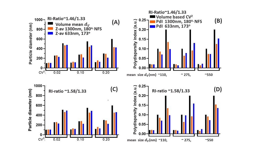
Fig. 5 Comparison of DLS data for the NFS at 1300nm (180o) with DLS at 633nm (173o). (A): Z-av data compared to the volume-based mean size dv (black) (B) Polydispersity Index PdI compared to the volume-based polydispersity (CoV)2 (black bars). Both (A) and (B) are for low RI-ratio ~1.46/1.33 e.g. lipid droplets in water. (C) and (D) show similar data as (A) and (B), but for a NP suspension with higher RI-ratio~1.58/1.33, representative for polystyrene or pharmaceutical NPs in water. Source: InProcess-LSP
For NPs with dv ~550nm, the reduction of the Z-av compared to dv for the two wavelengths are similar: both differences increase with polydispersity and Mie effects for both wavelengths (see Fig.4B,C) have a similar effect on the Z-av. Note that Z-av values less than dv contrast the common perception that the intensity-based Z-av should exceed dv, which is typical only for particle sizes in the Rayleigh regime. The corresponding PdI data (Fig5. B, D, last group) show that for a polydispersity (CoV)2=0.1 and 0.2, the difference between ‘measured’ PDI and (CoV)2 for the two wavelengths in fact depends on the RI-ratio, with a smaller difference for the 1300nm data when the RI-ratio is enhanced.
A careful look at how PdI data for (CoV)2=0.1 in Fig.5D (for one wavelength) vary with particle size, shows an oscillating effect in the ratio PdI /(CoV)2 on increasing size. A similar effect occurs for the ratio between Z-av and dv versus size in Fig.5D. This directly relates to the Mie resonances in Fig.3 and highlights the difficulties these resonances cause in interpreting DLS intensity-based size characteristics. In this respect, the ‘delayed’ onset of the Mie regime (i.e. at larger particle size) for the NanoFlowSizer SR-DLS system with λ=1300nm compared to backscatter systems at visible wavelengths, clearly facilitates the interpretation of NFS data with respect to volume-based results.
Finally, note that the relations between volume and intensity data in Fig. 5 apply only for lognormal volume PSDs. Other distributions yield different results, especially for bimodal PSDs, see also [9]. Therefore, more reliable analyses of volume-based PSD data from DLS are eventually the optimal way for the comparison of data from different instruments. Aside from more complicated/less practical ‘many angle’ approaches as in [10]. Such analyses benefit from (i) DLS correlation functions with the lowest possible noise levels (ii) limiting effects of Mie resonances (iv) analysis algorithms for volume PSDs using Mie theory at the appropriate level and (iii) accurate data on particle and solvent RI. The SR-DLS technology of the NFS, which measures a mean correlation function from up to ~1000 simultaneously depth-resolved data over a large total scattering volume, shows optimally low noise levels, as well as enhanced Rayleigh scattering range as discussed. Besides the unique high turbidity and flow capabilities for process analysis, the NFS thus also has significant benefits as off-line (lab) instrument.
Conclusion
DLS is an effective technique for rapid measurement of size and size dispersity of nanoparticles in suspensions. To overcome limitations of current standard instruments to measure highly turbid and flowing suspensions, e.g. for process monitoring, the NFS system with Spatially Resolved DLS has been developed, based on 180o backscattered Low Coherence Near InfraRed light, different from standard instruments. In this contribution we specifically address the question: How can particle size characteristics measured using different DLS instruments be compared to each other?
Practically, the answer is: when using only intensity-based Z-av and PdI data, without knowledge of the particle size distribution, it is very difficult to make a meaningful comparison between DLS data at different wavelengths or detection angles, except for very monodisperse suspensions (CoV<~0.1) such as reference standards. Comparison of more polydisperse suspensions might be possible when it is assured that the relevant size range stays within maximally ~0.2 of the wavelength (Rayleigh scattering). Beyond this range, comparing measurements on non-monodisperse NPs from different DLS systems, requires the full PSD information and careful accounting for Mie theory to derive volume-based PSD’s from DLS correlation functions. Low noise levels, use of NIR light and adequate algorithms that are features of the NanoFlowSizer system help in such comparison and data interpretation.
Methods
Lognormal volume-based PSD data with specified relative standard deviation ‘CoV’ (generated as in Fig 4a) are converted to theoretical intensity distributions Iλ,θ,m (d) using Mie theory for the specified suspension RI-ratio (m = np/ns), instrument-specific size ratio d/λ' and scattering angle θ. To simulate DLS-measured data, the intensity distribution is used to calculate the DLS first-order autocorrelation function g1 (τ) = ∑d Iλ,θ,m (d) ⋅ e -q2D(d)τ, using the Stokes-Einstein form D(d) = kBT/3πηd and scattering vector q=4 π/(λ/ns) ⋅ sin(θ/2) [11]. Subsequent cumulant analysis on g1 (τ) is performed [7] to obtain the ‘measured’ cumulant Z-av-and PdI, while the DLS Intensity-based PSD is obtained from regularized Laplace inversion (Non Negative Least Squares, e.g. [12]), of g1 (τ), as also employed in the NanoFlowSizer’s XsperGo software.
References
[1] J. Stetefeld, S. A. McKenna, and T. R. Patel, “Dynamic light scattering: a practical guide and applications in biomedical sciences,” Biophysical Reviews, vol. 8, no. 4. Springer Verlag, pp. 409–427, Dec. 01, 2016. doi: 10.1007/s12551-016-0218-6.
[2] R. Besseling, M. Damen, J. Wijgergangs, M. Hermes, G. Wynia, and A. Gerich, “New unique PAT method and instrument for real-time inline size characterization of concentrated, flowing nanosuspensions,” European Journal of Pharmaceutical Sciences, vol. 133, pp. 205–213, May 2019, doi: 10.1016/j.ejps.2019.03.024.
[3] A. Einstein, “On the motion of small particles suspended in liquids at rest required by the molecular-kinetic theory of heat,” Ann Phys, vol. 17, no. 549–560, p. 208, 1905.
[4] H. C. van de Hulst, Light Scattering by Small Particles. 1957.
[5] G. Mie, “Beiträge zur Optik trüber Medien, speziell kolloidaler Metallösungen,” Ann Phys, vol. 330, no. 3, pp. 377–445, 1908, doi: 10.1002/ANDP.19083300302.
[6] X. Cao, B. C. Hancock, N. Leyva, J. Becker, W. Yu, and V. M. Masterson, “Estimating the refractive index of pharmaceutical solids using predictive methods,” Int J Pharm, vol. 368, no. 1–2, pp. 16–23, Feb. 2009, doi: 10.1016/J.IJPHARM.2008.09.044.
[7] D. E. Koppel, “Analysis of Macromolecular Polydispersity in Intensity Correlation Spectroscopy: The Method of Cumulants,” J Chem Phys, vol. 57, no. 11, p. 4814, Sep. 1972, doi: 10.1063/1.1678153.
[8] B. J. Frisken, “Revisiting the method of cumulants for the analysis of dynamic light-scattering data.,” Appl Opt, vol. 40, no. 24, pp. 4087–4091, 2001, doi: 10.1364/AO.40.004087.
[9] L. Jin, C. W. Jarand, M. L. Brader, and W. F. Reed, “Angle-dependent effects in DLS measurements of polydisperse particles,” Meas Sci Technol, vol. 33, no. 4, p. 045202, Apr. 2022, doi: 10.1088/1361-6501/ac42b2.
[10] G. Bryant and J. C. Thomas, “Improved Particle Size Distribution Measurements Using Multiangle Dynamic Light Scattering,” Langmuir, vol. 11, no. 7, pp. 2480–2485, Jul. 1995, doi: 10.1021/LA00007A028/ASSET/LA00007A028.FP.PNG_V03.
[11] G. Bryant and J. C. Thomas, “Improved Particle Size Distribution Measurements Using Multiangle Dynamic Light Scattering,” Langmuir, vol. 11, no. 7, pp. 2480–2485, May 2002, doi: 10.1021/la00007a028.
[12] A. R. Roig and J. L. Alessandrini, “Particle Size Distributions from Static Light Scattering with Regularized Non-Negative Least Squares Constraints,” Particle & Particle Systems Characterization, vol. 23, no. 6, pp. 431–437, Dec. 2006, doi: 10.1002/PPSC.200601088.